ILE Matrices
The spectrum of a matrix tells you a lot. Eigenvalues and matrix entries are directly related by the determinant - but trying to grasp spectral information by eyeing individual entries is not sane.
$$\det (\lambda I - A) = 0$$
$\lambda$, the eigenvalues of $A$. Roots of $\det(A)$
Eigensystems curiously interlace individual entries and respond in surprising ways from small perturbations. For that reason, a video on matrices whose eigenvalues are integer-linear combinations of their entries caught my interest. I was left with many questions, so this here troglodyte brain poked around a bit.
$$det(A) = \sum_{i=1}^{n}(-1)^{i+j}a_{i,j}M_{i,j}$$
$$det(A) = \sum_{\sigma \in S_{n}}^{}\big(sgn(\sigma)\prod_{i=1}^{n}a_{i,\sigma(i)}\big)$$
The cofactor expansion and its unrolled counterpart below relating the determinant to individual matrix entries. The intuition for how single entries in relation to others contribute to the full spectrum is convoluted.
Researchers find subsets of matrices from the following construction:
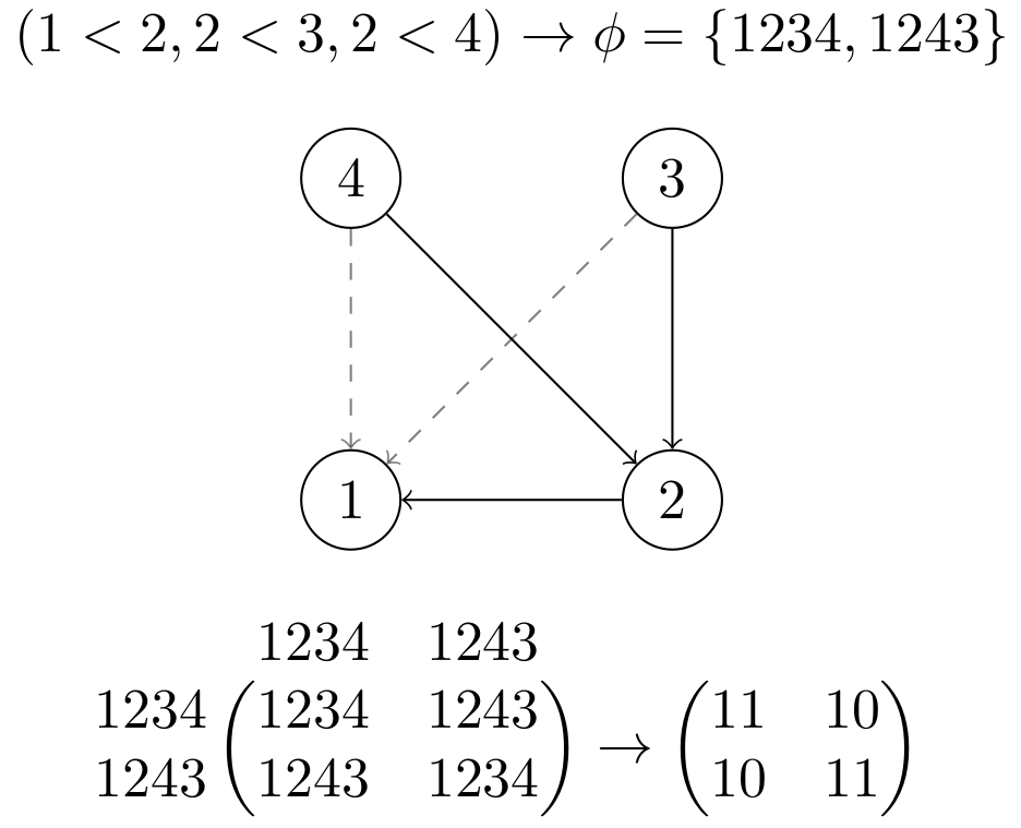
- Select a finite strict partial order (Fig. 1)
- Determine size-n permutations phi which satisfy said order
- Create a matrix whose (i,j) entries are $ \phi_{i}\phi_{j}(id) $
- For each entry, convert into a binary string marking increases or decreases in the sequence. For example, $132 \rightarrow 10$

Fig. 1: the partial order defined by the relations $(1<2, 2<3, 2<4)$ on an $n=4$ size system (transitive completion dashed). A partial order applies inequality constraints to a list of elements. In this case, two permutations satisfy the order.
You probably won't see a miracle by choosing a random order, and computing eigenvalues gets hard quick. So as a first stab we could filter for partial orders whose permutation's squares are all equal to one another to make the matrix diagonal have equal entries and increase the odds of seeing nice examples. We can find a more general way later.

A 9*9 matrix with integer-linear eigenvalues.
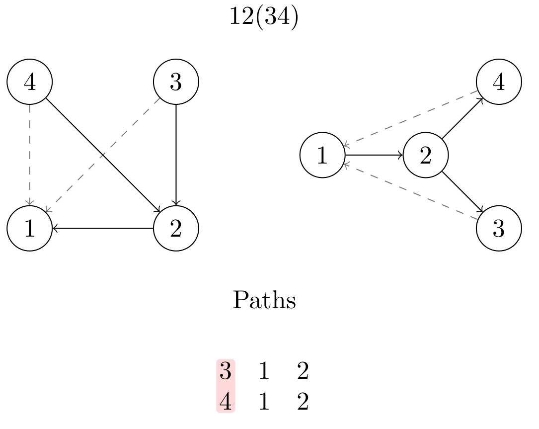
For these orders what kind of permutations are squares of themselves? Well, applying a permutation twice returns the elements to their starting positions, so it must only contain disjoint transpositions (non-overlapping swaps). Let's look at these orders graphically.

Fig 2: Order as a graph. Its permutations can be read from the existing paths.
Stacking the order's paths (Fig. 2) we can see shared vertices are fixed nodes and variable entries at an index are 2-cycles. Fixed nodes form a chain amongst themselves and free nodes wire to the start of fixed chains to section off their movement. Chains can enclose free regions like in $1(23)4$ (not to be confused with cycle notation - I am just enclosing swappable elements in parentheses) as we see the same chains at $1$ and $4$ and gap $x$ in paths $1\text{ }x\text{ }4$. Multiple disjoint regions or blocks like $1(23)(45)$ are no different, and by node relabeling we can consider all swaps to be local swaps. Expanding from matrices with constant diagonals to ones whose permutations allow non-disjoint local swaps, a block (block-motif) allows non-disjoint swaps on a subset of elements. Above we had 2-element blocks such as $(12)$ in an order like $(12)3$, but 3-blocks like $1(234)5$ ensure $2<4$ while the suborder indexed by $(234)$ has no other entries/edges. Non-disjoint means some legal swaps overlap, here $(23)$ and $(34)$. A b-block has b-1 overlapping 2-blocks - $(1(2)3)$. Elementary block dimensions of this slight expansion are the Fibonacci terms. A b-block yields $fib(b)$ permutations (its dimension), and the product of of each disjoint block's dimensions yields an order's resulting matrix size. Using || for cardinality, $fib(|(12)|)=fib(2)=2$ since $(12) \rightarrow | \lbrace 12, 21 \rbrace | = 2$. fib(|(1(2)(3)4)|)=fib(4)=5.$$\begin{matrix}112358... n \\ \text{ }012345... b\end{matrix}$$
The term elementary refers to the fact that a matrix constructed from non-disjoint local permutations must be a product of elementary block dimensions $\in fib()$, while prime blocks are $\in \mathbb{P} \cap fib()$. Unique elementary factorizations describe the number of ways we can reach a matrix of a given dimension. Given $k$ blocks of dimensions $b_i$, let $e$ and $p$ be the unique dimensions of the $k$ blocks and their respective frequencies. The number of arrangements of the given blocks over $n$ fixed elements (the # of such partial orders) is $$x=\frac{\prod\limits^{k}_{i=1}(n-(\sum\limits^{k}_{j=1}b_j-i))}{\prod\limits^{|p|}_{i=1}p_{i}!}$$ You can think of it as a modified combinatorial problem of putting balls into bins. The denominator accounts for symmetries in block assignments ($212$ has repeating assignments). For example when $k=2$ blocks of size $b=\lbrace 3,2 \rbrace$, we have $x=(n-4)(n-3)$, or $b=\lbrace 2,2 \rbrace$ yields $x=\frac{(n-3)(n-2)}{2}$. If I have $k=3$ blocks $\lbrace 6,2,2 \rbrace$ then $x=\frac{(n-9)(n-8)(n-7)}{2}$, and so on. The initial construction does not actually span the space of stochastic matrices with integer-linear eigenvalues. Even then, are the stochastic integer-linear eigenvalue matrices still just a subset?

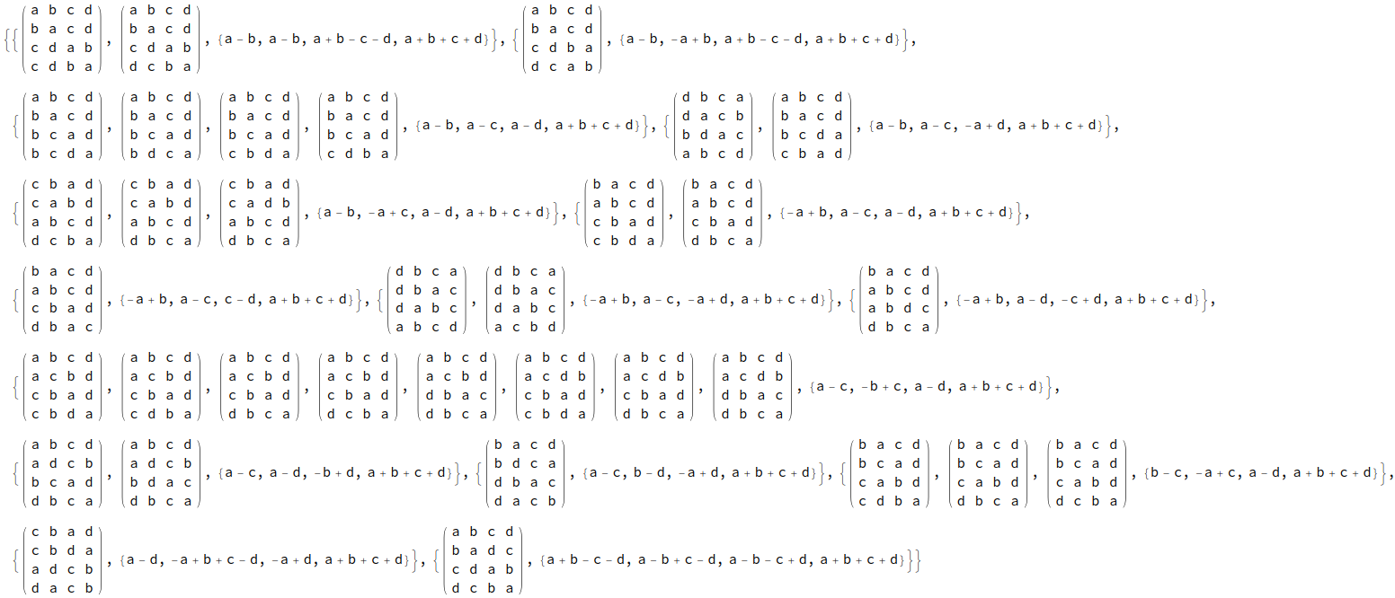
Fig. 3: The set of all compatible full-rank 3*3 row-stochastic matrices up to isomorphism, transpose, and variable relabeling (there are 10 of any rank)

Fig. 3b: Same set, but 4*4 matrices & sorted by their eigenvalues.
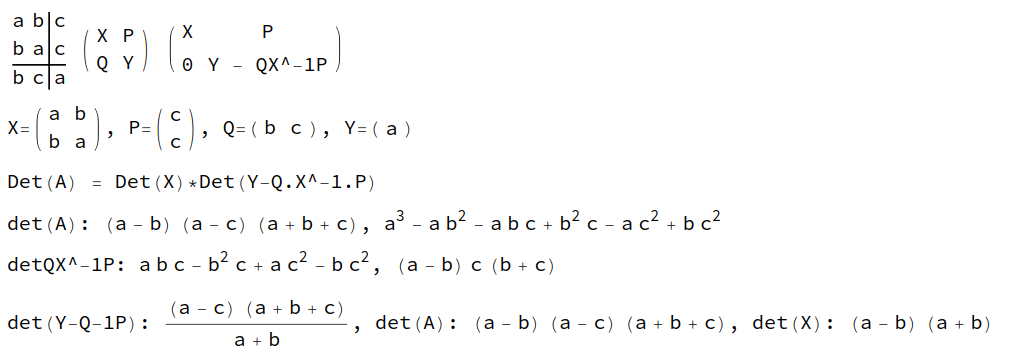
We can rewrite the resultant matrix $A$ as a $2*2$ partitioned matrix $$\begin{pmatrix} X & P \\ Q & Y\end{pmatrix}$$ and exploit Schur's complement for invertible X to compute $\det(A) = \det(X)*\det(Y - QX^{-1}P)$. Similar to how the unrolled cofactor expansion relates matrix entries to eigenvalues, we can recursively apply XPQY-block-partitions to make headway on 'why' ile matrices happen with the added benefit of a simpler determinant calculation that ties in the partial order's structure.

Fig. 4: Example decomposition and determinant calculation. Even for big $n$ you can choose a sub-block $X$ that is an ile matrix whose factors cancel from the inner contributing $X^-1$ term and outer $\det(X)$, while the remaining components form integer-linear factors and can conserve factors of $\det(X)$.
Working from a given partial order you can partition it anywhere that does not interrupt a given block to get submatrices that are valid ile matrices (Fig. 4). For example, $1(23)|4$ defines $n=3$ and $n=1$ ile submatrices, while $1(2|3)4$ does not. It's structurally nice to partition out large ile submatrices, which may require shuffling index labels around ($B =P^{-1}AP$ applies the same permutation to rows and columns, so it just shuffles the order of nodes in the partial order around). Submatrices on the diagonal will also be ile. There are definitely loose ends here, and a lot of interesting paths forward, but I thought it would be nice to leave the circle open in spirit of $\pi$ day. Working out the induction could be a satisfiable route to seeing how and why these miracles happen.